We won the 1st Prize, 1st Place at 4th Dean Fund Graduate Creative Innovation Contest. (presentation and news)
Technical Details
Let me introduce some technical details about road detection in severe shadow cases.
Task Definition. First we should define what does road detection do, here’s an example of road detection:
Road detection task
Given an image, we provide an pixel-wise annotation to show whether it belongs to road area or not. It’s worthwhile to mention some similar tasks like free space segmentation and semantic segmentation. Instead of finding road area, the goal of free space is to find areas that is drivable, say, ground area for a car, water area for a boat and so on. Most free space segmentation algorithms use radar data instead of image captured by a camera because these algorithms are focusing on collision avoidance and it’s the distance information that matters, which can be easily extracted from radar data. As for semantic segmentation, it attempts to partition the image into semantically meaningful parts, and to classify each part into one of the pre-determined classes. It involves the scene understanding, I mean, we need the context information and previous experience to find out the semantically meaningful parts. Therefore, it’s more complicated than road detection, which only deals with one specific class.
Problem Definition. One problem of road detection is, the illumination change. Although shadow on the road might provide information about object shape and location, it also introduce severe illumination changes, which might cause false alarms in Edge Detection, Texture Extraction and Color Segmentation.
Illumination Robust Feature
In this subsection, let me introduce the illumination robust feature extractor we proposed in ISM 2015.
Saturation
In RGB space, the brightness and color information are mixed together for three components, thus they are vulnerable to the impact of shadow. To solve this problem, color space conversion is often employed [11, 18, 20] to extract the brightness information into a separate component, such as I of HSI, L of Lab and Y of YUV. The remaining two components are suitable for road detection since they only contain color information which is relatively illumination-insensitive. Take HSI as an example, H component can be employed to extract road features [20], and S component is suitable to extract roadside vegetation [26].
As shown below, the S component is insensitive to the illumination changes:
Left: RGB image of road with weak shadows. Right: S component grayscale image.
The definition of S (saturation) is as follows: $$ S = \frac{\max(R,G,B) − \min(R,G,B)}{max(R,G,B)} $$ where S denotes the saturation of HSV color space and R, G and B denote the red, green and blue channels of the RGB color space respectively. Note that the saturation is defined to be zero when all channels of RGB are zero. Since the road surfaces are less colorful than the roadside vegetation, it has much lower S regardless of the illumination changes.
However, color components are unstable in severe shadow cases. We found the reason is that the road areas in server shadow show a little bit blue, which results in high S. (Why blue? ——I’ll explain it later)
Left: RGB image of road with severe shadows. Right: S component grayscale image.
Modified Saturation
To accommodate both the severe shadow cases and weak shadow cases, we proposed an illumination-robust feature called S’, which is defined as $$ S^\prime = \frac{\max(R,G,B) − B}{max(R,G,B)} $$ Such a slight modification, but it works! Since the road areas in server shadows have higher blue values, $\max(R,G,B) − B \approx 0$ ; while the road areas in weak shadows have small blue, that is, $\max(R,G,B) − B \approx \max(R,G,B) − min(R,G,B)$. In conclusion, the modification only works in server shadow cases, and fixes the high S to be low S.
Comparison
S and S’ in weak shadow cases.
S and S’ in severe shadow cases.
The feature extractor plays an important role in the road detection algorithm. Please read the paper for the whole algorithm implementation.
Shadow-Free Feature
In this subsection, I will introduce the shadow-free (or illumination invariant) feature extractor we proposed in MM 2016.
LCS Space
Since shadows still exist in the extracted component via illumination-robust extractors, the road boundary may not be recovered well in some cases [27]. To completely remove the shadow interferences, some researchers try to find underlying features which are invariant to illumination effects. Log-chromaticity space (LCS) [7] is often employed to recover a shadow-free image.
Before the introduction of our extractor, let me give a brief description of the existing extractors.
Under the condition that an image is captured by a narrow-band camera with approximately Planckian illumination and Lambertian surfaces, Finlayson et al.[7] show that the set of color surfaces of different chromaticities forms parallel straight lines in the LCS.
The band-ratio chromaticity is defined as $$ \chi_j := \frac{\rho_q}{\rho_p}, \quad q\in { 1,2,3}, q \neq p, \quad j = 1,2, $$ where ρ1 , ρ2 and ρ3 are matrices respectively representing the red(R), green(G) and blue(B) components of the raw image, p is the index of the normalizing components and index q points to the remaining two components. The shadow-free image I proposed in [7] is derived from the aforementioned linear relationship as $$ \mathcal{I} := \exp(\cos\theta \ln \chi_1 + \sin \theta \ln \chi_2), $$ where θ is a camera-dependent parameter.
Alvarez and Lopez [2] presents a sped up version where G is used for normalization (p = 2;q = 1,3) and the outermost exponential operation is removed to improve the speed. $$ \mathcal{I}_\theta := \cos \theta \ln (\frac{R}{G}) + \sin \theta \ln (\frac{B}{G}), $$
Maddern et al.[16] proposed another form of illumination invariant imaging and applied it to vision-based localization, mapping and classification for autonomous vehicles. Their extractor is defined as $$ \mathcal{I}_\alpha := (1-\alpha) \ln {R} +\alpha\ln B - \ln G + 0.5 , $$ where α is a camera dependent parameter ($\alpha = \frac{\sin \theta} {\cos \theta + \sin \theta}$) and 0.5 is an offset term.
shadow-free feature extractors perform better than illumination-robust extractors in weak shadow cases since the shadows are completely removed. However, their performance in severe shadow cases still needs to be improved. To find why existing shadow-free extractors [2,16] fail in severe shadow cases, we choose a shadowy road image from ROMA dataset [21] and then map pixels of road and vegetation regions into LCS. According to their basic assumption, the set of color surfaces of different chromaticities will form parallel straight lines in LCS. However, the distribution is more like a quadratic function in severe shadow conditions, and the two classes are mixed together indistinguishably.
Road and vegetation pixels on log(R/G)-log(B/G) plane
RGB Space
Instead of using LCS, we found that the linear relationship in RGB space is more reliable. As shown below, the road and vegetable pixels are distinguishable in RGB space.
Road and vegetation pixels on G-B plane
So our feature extractor is defined as $$ \mathcal I_b := 2 - \frac{G-b}{B} $$ where b is a scene dependent parameter (we used to think it is a camera dependent parameter, but it actually not, I’ll detail it later).
We test three edge detectors (Sobel, Canny and Structured Edge) in severe shadow cases. As shown in Fig.7, using the shadow-free image obtained by our extractor can achieve a better result.
Fig.7 Improve edge detection via our extractor.
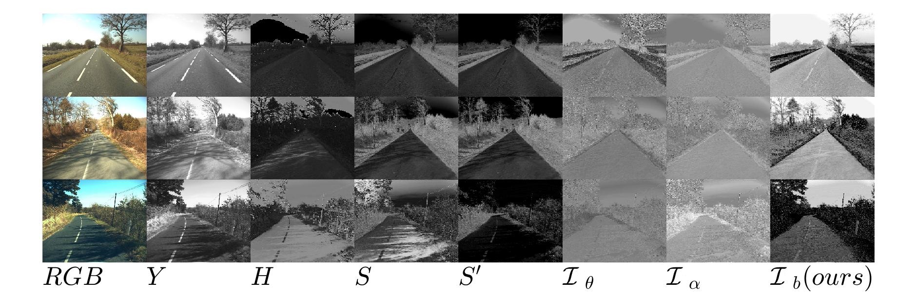
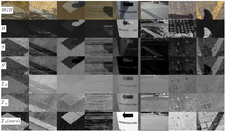
Comparison
Comparison of various feature extractors.
Shadowy images and the results of extractors
We also built an online demonstration here (implemented in Javascript).
Why it works
In this section, I’ll provide the physical explanation of the proposed methods.

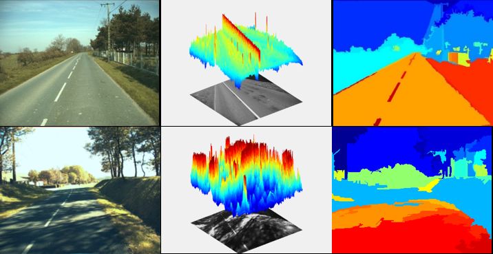
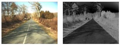
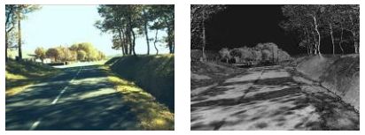
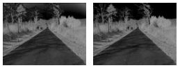
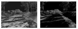
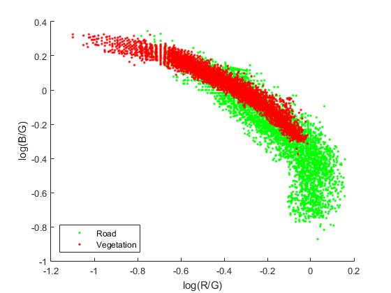
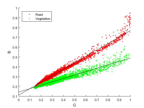
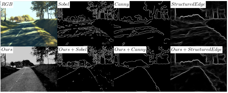 Fig.7 Improve edge detection via our extractor.